
Machine Learning with Clojure and Cortex
Machine Learning Clojure/Cortex
Never let formal education get in the way of your learning.
Mark Twain
Sometimes it’s not easy to start something new. Machine learning probably is one of those programming skills you need to insert in soon to go live project but you do not really know where to start with. Of course, You have already heard the hype, and know the skill should be on your resume but never really got started.
While some of the simple tutorials are in the Python programming language, this short paper will be on using Clojure and Cortex for Machine Learning will allow you to create from scratch easy to understand neural networks ready for use, and also be able to get instant results from your trained network using the REPL dear to LISP.
Cortex is new, but a very strong alternative to existing Machine Learning framework. The fact that is Clojure based, removes most of the surrounding boiler plate code required to train and run.
Some examples I have created in the past with Cortex were used to classify cats and dogs:
https://github.com/thinktopic/cortex/tree/master/examples/catsdogs-classification
or a large set of fruits:
http://blog.hellonico.info/clojure/using_cortex/
and while both posts, either with dogs and cats, or fruits present how to write a neural network for images classification, with this entry we would like to go to the root of things and show you how to do write an even simpler, but still effective, network in a few lines.
To highlight how to train and use the network, we will create a simple secret function, secret to the network that is, and we will train the network so to be able to compute inputs it has never seen before, with quite very good results.
Cortex itself is a Clojure library that provides APIs to create and train your own network, including customizing input, output, and hiddent layers, along having an estimate on how good or bad the current trained network is.
The minimal Clojure projet setup is a quite a standard Leiningen setup. We will make use of the library thinktopic/experiment which is a high-level package of cortex library.
 {width=“3.345227471566054in” height=“1.5896423884514437in”}
We will also use one of my favourite, the Gorilla REPL, so to have a web REPL along plotting functions, that we will use later on.
(defproject cortex-tutorial "0.1-SNAPSHOT"
  :plugins [[lein-gorilla "0.4.0"]]
  :aliases {"notebook" ["gorilla" ":ip" "0.0.0.0" ":port" "10001"]}
  :dependencies [[org.clojure/clojure "1.8.0"]
  [thinktopic/experiment "0.9.22"]])
The gorilla plugin allows to run a Web REPL, and you can start it by using the notebook alias provided in the above project.clj file. And so, as a simple terminal or console command:
lein notebook
You are all setup and ready to get going. In a Clojure namespace, you are going to define three things.
One is the secret function that the network will be supposed to map properly.
The second is a generator for a sequence of random input.
The third is data set generator, to provide the network for training. This will call the secret-fn to generate both the input and output required to train the network.
In the project attached to this post, this Clojure namespace is defined in src/cortex_tutorial.clj and will be used via the two Gorilla notebooks.
(ns cortex-tutorial)

(defn my-secret-fn [ [x y] ]
  [ (* x y)])

(defn gen-random-seq-input [rand-fn]
  (repeatedly (fn[][(rand-fn 10) (rand-fn 10)] )))

(defn gen-random-seq []
  (let[ random-input (gen-random-seq-input rand-fn)]
  (map #(hash-map :x % :y (my-secret-fn %)) random-input)))
With the Gorilla REPL started, head to the following local URL:
http://127.0.0.1:10001/worksheet.html?filename=notebooks/create.clj
This is where the REPL is located, and where you can follow along the notebook and type Clojure code and commands directly in the browser.
Preparation
The first thing is to import some namespaces.
(ns frightened-resonance
(:require
  [cortex.experiment.train :as train]
  [cortex.nn.execute :as execute]
  [cortex.nn.layers :as layers]
  [cortex.nn.network :as network]
  [tutorial :as tut] :reload))
The network and layers namespaces will be used to define the internals of your network. The train namespace takes the network definition and datasets to produce a trained network. Finally, the execute namespace takes the trained network and an extra input only dataset to run the network with the provided input. The tutorial namespace contains the code written above, with the hidden function and data sets generators.
Creating and testing the input generators will be your first step. The input generate produces a number of tuples made of 2 elements each.
(into [] (take 5 (tut/gen-random-seq-input)))
; [[9 0] [0 4] [2 5] [5 9] [3 9]]
The random-seq generate can provide datasets with both input and output, internally using the hidden function.
(into [] (take 5 (tut/gen-random-seq)))

; [{:y [3], :x [1 3]} {:y [6], :x [3 2]} {:y [0], :x [0 2]}
{:y [15], :x [3 5]} {:y [30], :x [6 5]}]
Now that you get an idea of what the generated data looks like, let’s create two data sets, both of 20000 elements. The teach-dataset will be used to tell the network what is known to be true, and it should learn as is, while the test-dataset will be used to indeed test the current correctness of the network, and compute its score. It is usually better to have two different sets.
(def teach-dataset
  (into [] (take 20000 (tut/gen-random-seq))))

(def test-dataset
  (into [] (take 20000 (tut/gen-random-seq))))
Strong of two fantastic data-sets, let’s write your network. The network will be defined as a common linear-network, made of 4 layers.
Two layers will be for the expected input and output, while two other layers will define the internal structure. Defining the layers of a network is quite an art in itself, here we take the hyperbolic tangent activation function. I actually got a better trained network by having two tanh based activating layers.
See https://theclevermachine.wordpress.com/tag/tanh-function/ for a nice introduction on this topic.
The first layer defines the entrance of the network, its input, and tells that there are 2 elements as 1 input, and that the label of the input is named :x.
The last layer defines the output fo the network, and tells there is only one element and that its id will be :y.
Using the Cortex api, this gives the small network code below:
(def my-network
(network/linear-network
 [(layers/input 2 1 1 :id :x)
  (layers/linear->tanh 10)
  (layers/tanh)
  (layers/linear 1 :id :y)]))
All the blocks required to train the network are defined, so as the Queen would say…
It’s all to do with the training: you can do a lot if you’re properly trained.
Queen Elizabeth II
Training
The goal of training is to have your own trained network, that you can either use straight away, or give to other users so they can use your network completely stand alone.
Training is done in steps. Each step takes elements of the teaching dataset in batch, and slowly fit the blocks of each layers with some coefficients, so the overall set of layers, can give a result close to the expected output. The activation functions we are using, are in some sense mimic-ing the human memory process.
After each teaching step, the network is test-ed for its accuracy using the provided test-dataset. At this stage, the network is run with the current internal cofficients, and compared with a previous version of itself, to know whether it performs better or not, computing something known as the loss of the network.
If the network is found to be better than its last iteration, Cortex then saved the network as a .nippy file, which is a compressed version of the network represented as a map. Enough said, let’s finally get started with that training.
(def trained
  (binding [*out* (clojure.java.io/writer "my-training.log")]
  (train/train-n my-network teach-dataset test-dataset
    :batch-size 1000
    :network-filestem "my-fn"
    :epoch-count 3000)))
The output of the training will be in the log file, and if you look the first thing you can see in the logs is how the network is internally represented. Here the different layers, with the input and output sizes for each layer, and the number of parameters to fit.
Training network:
| type | input | output | :bias | :weights |
|---------+-------------+-------------+-------+----------|
| :linear | 1x1x2 - 2 | 1x1x10 - 10 | [10] | [10 2] |
| :tanh | 1x1x10 - 10 | 1x1x10 - 10 | | |
| :tanh | 1x1x10 - 10 | 1x1x10 - 10 | | |
| :linear | 1x1x10 - 10 | 1x1x1 - 1 | [1] | [1 10] |
Parameter count: 41
Then for each step, or each epoch goes the new score, and whether or not the network was better, and in that case saved.
| :type | :value | :lambda | :node-id | :argument |
|-----------+-------------------+---------+----------+-----------|
| :mse-loss | 796.6816681755391 | 1.0 | :y | |
Loss for epoch 1: (current) 796.6816681755391 (best) null
Saving network to my-fn.nippy
The score of each step gives the effectiveness of the network, and the closer the loss is close to zero, the better the network is performing. So, while training your network, you should be looking to get that loss value as low as possible.
The full training with 3000 epochs should only take a few minutes, and once done you can immediately find out how our trained network is performing. If you are in a hurry, 1500~2000 is a good range of epochs that already makes the trained network quite accurate.
Once the training is done, you will find a new my-fn.nippy file in the current folder. This is a compressed file version of the cortex network.
A copy of the trained network, mynetwork.nippy, has been included in the companion project. The loss of the network was pretty good, with a value very close to zero as seen below.
Loss for epoch 3000: (current) 0.031486213861731005 (best)
0.03152873877808952
Saving network to my-fn.nippy
Let’s give our newly trained network a shot, with a manually defined custom input.
(execute/run trained [{:x [0 1]}])
; [{:y [-0.09260749816894531]}]
Which is quite close to the expected 0*1=0 output.
Now, let’s try something that the network has never seen before, with a tuple of double values.
(execute/run trained [{:x [5 1.5]}])
; [{:y [7.420461177825928]}]
Sweet. 7.2 is quite good compared to the expected result: 5*1.5=7.5
Using the network
Now, as you saw, the trained network was saved in a nippy file. That file can be loaded and used by “users” of your network. From now on, if you look at the provided notebooks, you can load the following note:
http://127.0.0.1:10001/worksheet.html?filename=notebooks/use.clj
The users will be needing a few namespaces. The tutorial and execute namespaces you have seen before, util will be used to load the network from a file, and plot is provided by gorilla to plot values and we will plot the expected results versus the network provided results.
(ns sunset-cliff
(:require
  [cortex.nn.execute :as execute]
  [cortex.util :as util]
  [tutorial :as tut]
  [gorilla-plot.core :as plot]
  :reload))
Loading the trained network is a simple matter of using the read-nippy-file provided by Cortex.
(def nippy (util/read-nippy-file "mynetwork.nippy"))
We did not look at it before, but the network is indeed a map, and you can check its top-level keys.
(keys trained)
; (:compute-graph :epoch-count :traversal :cv-loss)
And it is usually a good idea to check the number of eopchs the network has been going through, along with its current loss value.
(select-keys trained [:epoch-count :cv-loss])
; {:epoch-count 3000, :cv-loss 0.030818421955475947}
You can confirm the loaded network is given the same result as its freshly trained version from the last section.
(execute/run trained [{:x [5 1.5]}])
; [{:y [7.420461177825928]}]
Now, let’s generate a bunch of results with the loaded network and plot them. Running the network on a fresh input set is now trivial for you.
(def input (into [] (take 30 (tut/gen-random-seq))))
(def results (execute/run trained input))
And, of course, we can check a few of the result values produced by the network.
(clojure.pprint/pprint (take 3 results))
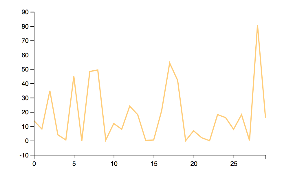
Plotting can be done using the Gorilla provided plotting functions, from the gorilla-plot.core namespace. Here, we will take interest only in the output, and we will use clojure’s flatten to create a flat collection, as opposed to the sequence of vectors found in the results.
(plot/list-plot (flatten (map :y results))
 :color "#ffcc77"
 :joined true)
After specifying a color, and the fact that plot should use lines instead of dots, you can see straight in the browser REPL, the graph below.
 {width=“2.8949650043744533in” height=“1.7400656167979003in”}
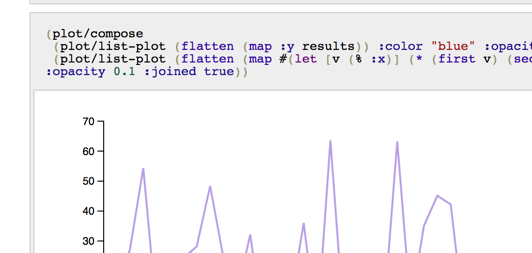
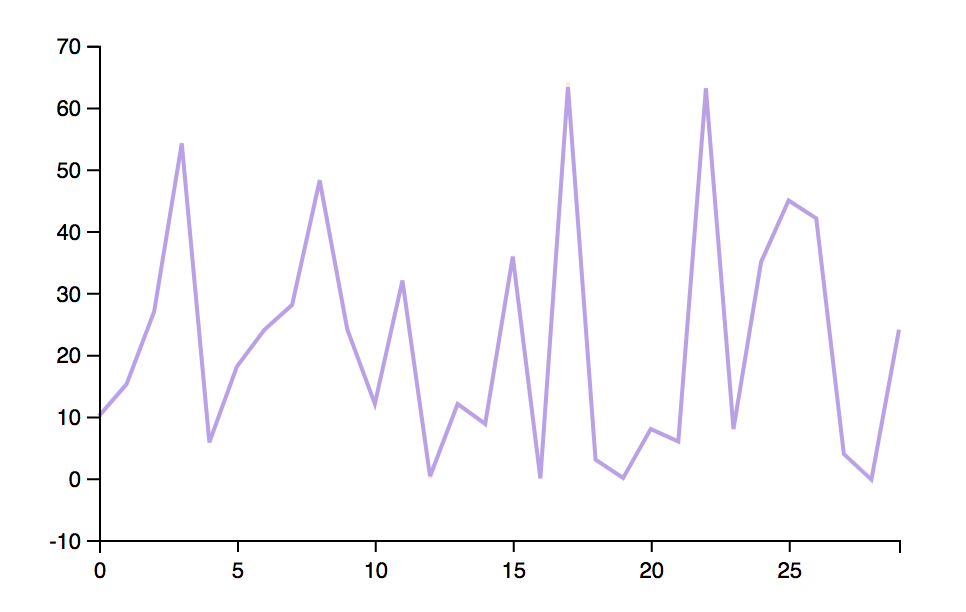
And you can also produce a “composed” graph, made of the expected results produce straight from the known or not hidden function, versus results produced by the trained network.
(plot/compose
  (plot/list-plot
   (flatten (map :y results))
   :color "blue"
   :opacity 0.3
   :joined true)
  (plot/list-plot
   (flatten (map #(let [v (% :x)] (* (first v) (second v))) input))
   :color "blue"
   :opacity 0.3
   :joined true))
And the two lines are actually too close, and so quite overlap each other.
 {width=“3.1417344706911634in” height=“1.98794728783902in”}
Re-train
From there an interesting progression path would be to take the currently trained network, and make it better by using more datasets, and running the cortex train-n function again.
(require '[cortex.experiment.train :as train])
(def teach-dataset
  (into [] (take 200 (tut/gen-random-seq))))
(def test-dataset
  (into [] (take 200 (tut/gen-random-seq))))

(def re-trained
  (binding [*out* (clojure.java.io/writer "re-train.log")]
   (train/train-n trained teach-dataset test-dataset
     :batch-size 10
     :network-filestem "retrained"
     :epoch-count 10)))
Note, that by specifying a new network-filestem you can keep a separate version of the updated network.
And, with the new datasets, and the new training cycle, there is still a chance to train to a better network.
Loss for epoch 3012: (current) 0.03035303473325996 (best)
0.030818421955475947
Saving network to retrained.nippy
From here to …
You have seen in this post how to train your own network to simulate the output of a know function.
You saw how to generate and provide the required datasets used for training, and how cortex saves a file version of the best network.
You saw how to
Now, some ideas would be to:
- Try the same for a different hidden function of your own
- Change the number of input and output parameters of the function, and the network in the network metadata.
- If the network does not perform as well as expected, it will be time to spend some time on the different layers of the network and find a better configuration.
The companion project can be found on github: